Bonus Payout Curve Generator
A parametric payout-curve generator tuned by a genetic algorithm to hit a target budget utilization while keeping engagement inside a stakeholder-defined band.
Designing a fair bonus curve is a six-parameter, non-convex problem - start/mid/max points and bonuses all interact, and the curve must respect budget while sustaining engagement.
Piecewise fit: exponential growth from start→mid, saturation growth from mid→max. Wrap it in a DEAP GA that drives budget utilization toward 100% (minimizing |100 − utilization|) with penalties for engagement out of band.
Utilization climbed from 85.5% → 93.4% at a clean 90.0% engagement rate. Manual judgment replaced by a reproducible, auditable calibration.
Before optimization
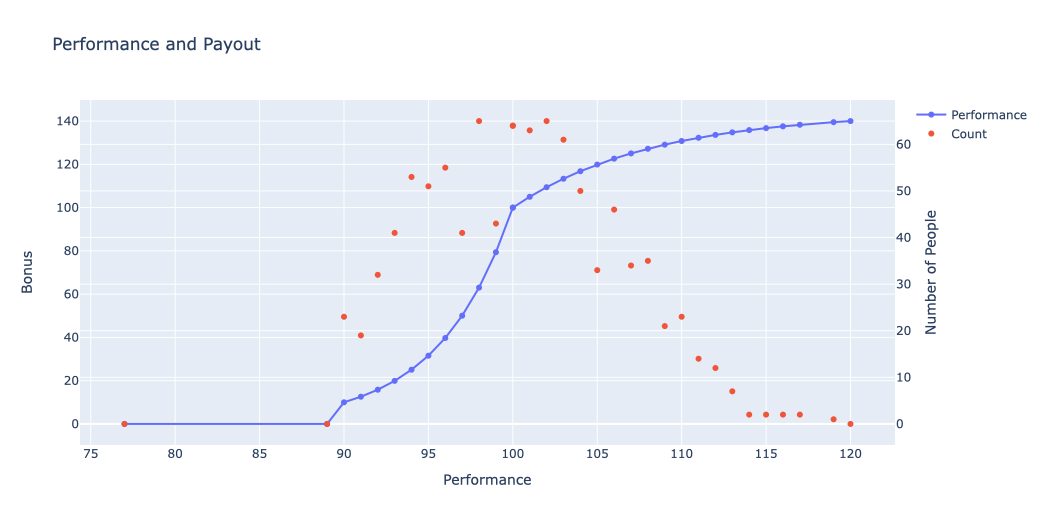
| P | Bonus % | Perf % |
|---|---|---|
| 10 | 19.91 | 93.0 |
| 20 | 31.55 | 95.0 |
| 30 | 50.03 | 97.0 |
| 40 | 79.38 | 99.0 |
| 50 | 100.00 | 100.0 |
| 60 | 108.53 | 101.8 |
| 70 | 113.34 | 103.0 |
| 80 | 119.90 | 105.0 |
| 90 | 127.19 | 108.0 |
| 100 | 139.50 | 119.0 |
GA-tuned parameters
100 individuals · 50 generations · tournament select (k=3) · two-point crossover · uniform-int mutation (indpb=0.2) · DeltaPenalty for monotonicity infeasibility.
After optimization
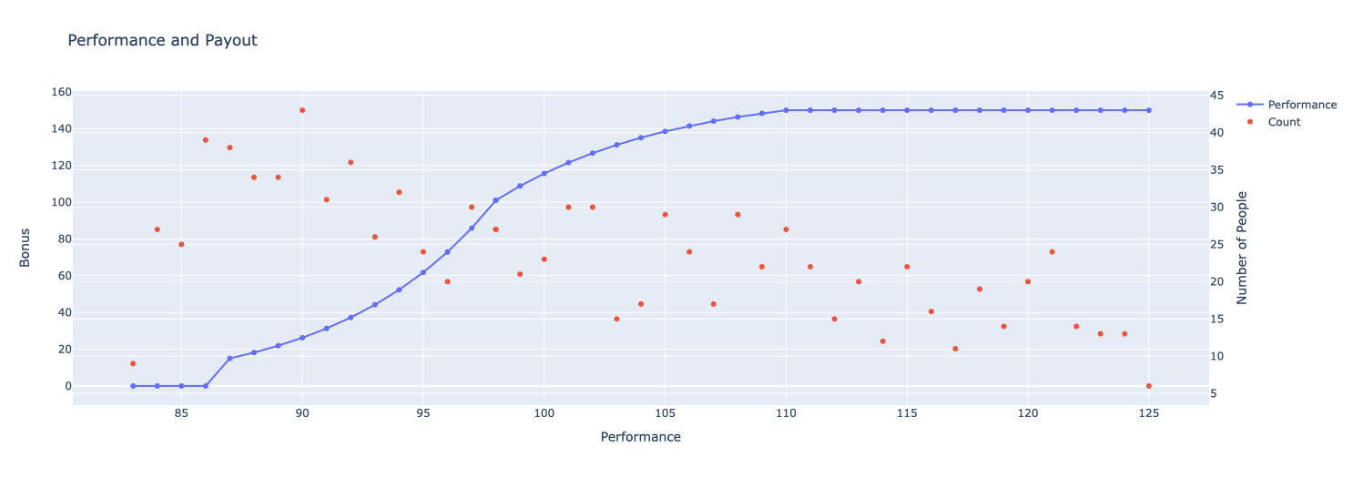
| P | Bonus % | Perf % |
|---|---|---|
| 10 | 15.00 | 87.0 |
| 20 | 22.76 | 89.2 |
| 30 | 37.25 | 92.0 |
| 40 | 72.88 | 96.0 |
| 50 | 108.80 | 99.0 |
| 60 | 131.16 | 103.0 |
| 70 | 146.32 | 108.0 |
| 80 | 150.00 | 112.0 |
| 90 | 150.00 | 119.0 |
| 100 | 150.00 | 125.0 |
Methodology
1. Piecewise curve fit
Performance below start_point → 0 bonus. Above max_point → capped at max bonus. Between, two regimes:
def fit_exponential(self, x, y):
    log_y = np.log(y)
    m, c = np.polyfit(x, log_y, 1)
    exponent = np.exp(m)
return exponent**x * np.exp(c)def saturation_growth_model(self, x, L, k):
return L - (L - self.mid_bonus) * np.exp(
-k * (x - self.mid_point)
)
# fit with bounds and p0 around mid/max bonus
popt, _ = curve_fit(model, x, y,
p0=(max_bonus, 1e-3),
bounds=([mid_bonus, 0], [max_bonus, 10]))2. Objective & feasibility
Objective = |100 − budget_utilization| — the absolute gap to a 100% spend target, so over-spend and under-spend are both penalized. Engagement-rate violations add a fixed penalty. Monotonic ordering of points/bonuses enforced via DEAP's DeltaPenalty.
def objective(x):
    sp, mp, xp, sb, mb, xb = np.array(x).round().astype(int)
    payout = PayoutGen(data, sp, mp, xp, sb, mb, xb, avg_bonus_amt).gen_payout()

    obj = abs(100 - payout.stats.budget_utilization)
    if not 80 <= payout.stats.engagement_rate <= 90:
        obj += 1000
    if payout.stats.meaningful_engagement_rate < 50:
        obj += 1000
    return obj

toolbox.register("evaluate", lambda ind: (objective(ind),))
toolbox.decorate("evaluate", tools.DeltaPenalty(feasible, 1000.0, distance))
toolbox.register("mate",   tools.cxTwoPoint)
toolbox.register("mutate", tools.mutUniformInt, low=lows, up=highs, indpb=0.2)
toolbox.register("select", tools.selTournament, tournsize=3)

algorithms.eaSimple(pop, toolbox, cxpb=0.7, mutpb=0.2, ngen=50)
3. Sensitivity analysis
For every candidate curve, sales are perturbed ±10% and attainment is re-bucketed against the fitted payout. The baseline curve was brittle (18% utilization at −10% sales); the optimized curve is more robust (51% utilization at −10% sales) at the cost of slightly higher upside exposure (127% vs 124%).